


Summary
Compressive sensing (CS) is a relatively new field that has generated a great deal of excitement in the signal-processing community. Research has applied CS to many forms of measurement, including radio detection and ranging (RADAR), light detection and ranging (LIDAR), magnetic resonance imaging (MRI), hyperspectral imaging, high-speed imaging, X-ray tomography, and electron microscopy. Benefits range from increased resolution and measurement speed to decreased power consumption and memory usage. CS has received mixed reviews in commercial and government circles. Some have touted CS as a cure-all that can be “thrown” at any sensor problem. Others consider CS all hype—just a rebranding of old theories. Who is right?
In order to answer this question, an overview of CS is presented, clarifying common misconceptions. Case studies are brought to illustrate the advantages and disadvantages of applying CS to various sensor problems. Guidelines are extracted from these case studies, allowing the readers to answer for themselves, “Can CS solve my sensor and measurement problems?”
Introduction
At first look, it appears that CS is widespread and revolutionizing a variety of sensor systems. Four new Institute of Electrical and Electronics Engineers (IEEE) paper classification categories have been created specifically for CS. Thousands of research papers have been published [1], representing significant academic funding by government and industry. The Wikipedia entry on CS [2] declares that “compressed sensing is used in a mobile phone camera sensor” and “commercial shortwave-infrared cameras based upon compressed sensing are available.” The infrared (IR) camera refers to InView’s single-pixel camera, a highly-publicized, real-world example of compressive sensing in action [3]. The MIT Technology Review article “Why Compressive Sensing Will Change the World” [4] explains how CS has supplanted the Nyquist-Shannon sampling theorem, a foundation in signal processing during the last century, and that CS is “going to have big implications for all kinds of measurements” [4].
A closer look, however, reveals some doubts about CS. There are anonymous comments, such as “Most of it seems to be linear interpolation, rebranded” [5] or “Compressed sensing…was overhyped” [6]. There are researchers like Yoram Bresler, a professor at the University of Illinois, that claim that CS is not really new. He asks, “Would a rose by any other name smell as sweet?,” claiming that CS is just a new name for earlier techniques, such as image compression on the fly and blind spectrum sampling [7].
Some CS researchers acknowledge shortcomings. Thomas Strohmer, a professor and the University of California Davis, asks, “Is compressive sensing overrated?” and notes that “the construction of compressive sensing based hardware is still a great challenge” [8]. Simon Foucart, a professor of mathematics at Texas A&M University, describes how “projects to build practical systems foundered…” and that “…compressed sensing has not had the technological impact that its strongest proponents anticipated” [9]. When asked what was holding CS back from imaging applications, Mark Neifeld, a professor at the University of Arizona, answered that “we haven’t discovered the ‘killer’ application yet” [10].
There are other scholars that are openly critical of CS. Leonid Yaroslavsky, a professor at Tel Aviv University and an Optical Society fellow, writes, “Assertions that CS methods enable large reduction in the sampling costs and surpass the traditional limits of sampling theory are quite exaggerated, misleading and grounded in misinterpretation of the sampling theory” [11]. In a section of his website titled “Fads and Fallacies in Image Processing,” Kieran Larkin, an independent researcher with 4,274 paper citations, declares that “everyone knew that the single-pixel camera research was a failure” [12]. He is referring to the InView single-pixel camera previously mentioned that was purported to be a successful application of CS. Who is right? Will CS bring about a revolution in sensing and measurement or is it really just all hype?
There are many tutorials [13–15], review papers [16–18], and articles [4, 19, 20] on CS, but they tend to be too technical or general for many readers. The technical sources are inaccessible to those without a signal processing background, while the nontechnical sources are too vague to give an intelligent perspective on CS. They do not address specific criticisms, leaving the readers on their own to judge between the supporters and detractors of CS. They are also generally written by CS researchers that may justly or unjustly be suspected of bias.
This article seeks to provide an accessible explanation of CS that gives enough background to examine claims and criticisms. In an effort to make CS understandable to the layman, concepts have been simplified, details have been glossed over, and equations have been replaced by intuitive explanations. For a more in-depth treatment of CS, several tutorials provide a good starting point [13–15].
Traditional Sampling
Overview
CS is sometimes referred to as compressive sampling since it is the sampling process that lies at the heart of CS. Sampling transforms continuous analog signals into discrete digital values that can be processed by a computer. In this age of low-cost computing, virtually all sensor systems sample signals, from commercial audio and video equipment to specialized medical and military systems. The speed or resolution at which a signal is sampled is called the sampling rate. Samples are typically taken at regular intervals, and the sampling rate determines the size of the features that can be identified in a signal. The more samples taken, i.e., the higher the sampling rate, the smaller the features that can be identified. When designing any system that samples data, the sampling rate must be carefully considered. If it is too high, the extra samples can increase power consumption, memory usage, computing complexity, and cost for little or no gain in performance. If it is too low, important information is lost, degrading performance, or even making the system unusable.
Nyquist-Shannon Sampling Theorem
In order to appreciate CS, we must first explain traditional sampling in some detail. The top left plot of Figure 1 shows a 1-Hz sinusoidal signal, i.e., there is one cycle per second. Such a signal could represent many different types of physical phenomenon, such as a voltage oscillating over time. The middle left plot shows a 10-Hz signal, i.e., 10 cycles per second. The bottom left plot shows the summation of these two signals. The top plot on the right shows this summed signal sampled at 10 Hz, i.e., 10 samples per second. This is an example of traditional sampling.
![Figure 1: An Example of Traditional Sampling (Source: U.S. Army Combat Capabilities Development Command Army Research Laboratory [CCDC ARL]).](https://www.dsiac.org/wp-content/uploads/2020/05/DSIACJournal_Spring2020_CompressiveSensing_Don_Fig1.png)
Figure 1: An Example of Traditional Sampling (Source: U.S. Army Combat Capabilities Development Command Army Research Laboratory [CCDC ARL]).
An analog-to-digital converter (ADC) would sample the signal at regular intervals 30x over the 3-s period to produce the samples marked as red dots. These samples are connected by a green line in an attempt to reconstruct the original signal. The reconstruction completely misses the 10-Hz signal, creating a waveform similar to the original 1-Hz signal. Clearly, the 10-Hz sample rate is too slow to detect the 10-Hz signal. The middle right plot shows the same signal sampled at 20 Hz, successfully capturing the 10-Hz signal.
The Nyquist-Shannon sampling theorem states that the sampling rate must be at least twice the highest frequency of a signal. This intuitively makes sense. In order to detect the important features of a signal, there needs to be at least one sample per feature. The important features of a sinusoid can be viewed as the valleys and peaks of each cycle. Therefore, two samples are needed per cycle. In this case, a 20-Hz sampling rate allows us to sample at the valley and peak of each cycle of the 10-Hz signal. The bottom right plot shows the boxed detail from the plot above it. The green lines connecting the samples give a good approximation of the signal but do not perfectly match the original waveform in blue. However, we will see that the signal can be perfectly reconstructed using sampling theory.
The signal in Figure 1 is relatively simple, just a combination of two sinusoids. A plot of the spectrum of this signal is shown in the top left plot of Figure 2. Instead of viewing the signal as a voltage oscillating in the time domain, the plot shows the amplitudes of the sinusoids that make up the signal in the frequency domain. The frequency domain is commonly referred to as the Fourier basis. The normal domain in which we typically view the signal, in this case, the time domain, is commonly called the standard basis. The idea of representing signals in different bases will be an important concept in CS that will be revisited later. The bottom left plot shows a more complicated spectrum with 14 nonzero values, corresponding to 14 sinusoids in the time domain that are summed to produce the signal in the top right plot. This signal is sampled above the Nyquist rate and reconstructed using sampling theory as the dashed red line in the bottom right plot, perfectly matching the original signal in blue. This is a remarkable result. A continuous analog signal composed of many frequencies that is sampled at the Nyquist rate can be perfectly reconstructed.
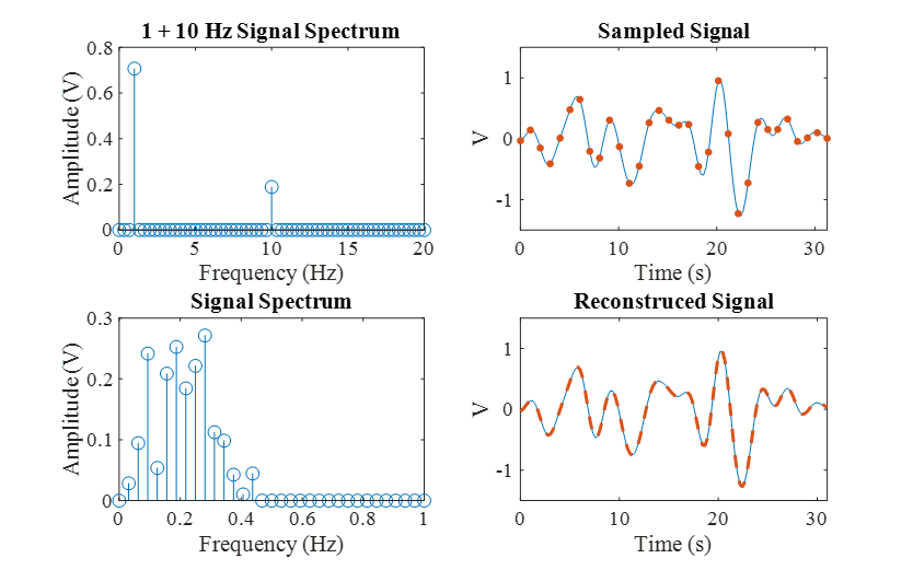
Figure 2: Sampling Example With Perfect Reconstruction (Source: CCDC ARL).
Two-Dimensional (2-D) Sampling
Figure 3 gives an example of 2-D sampling. In the case of one-dimensional (1-D) signals, one sensor (the ADC) samples at regular time intervals. In imaging, multiple sensors are typically spaced at regular intervals to create a 2-D sensor array. Just as the sampling rate determined the smallest detectable feature for the 1-D signal, the resolution of the 2-D array determines the smallest detectable features in the image. The relatively high-resolution image on the left is 1024 x 1024 pixels. The middle image shows the magnified detail of an airplane, with an ARL logo clearly recognizable. The right image has a resolution of 512 x 512, where the logo is now unrecognizable. The line width (i.e., feature size) of the letters was 1 pixel for the 1024 x 1024 array. When we decrease the resolution to less than 1 pixel per feature, those features become unrecognizable.
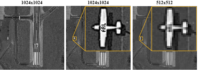
Figure 3: A 2-D Sampling Example (Source: CCDC ARL).
A Scanning Single-Pixel Camera
Images are typically sampled using a 2-D sensor array, but there are other methods as well. A single sensor could scan the scene, pixel by pixel, row by row, to acquire a complete 1024 x 1024 image. Figure 4 shows an example of such a system. A lens projects a scene onto a digital micromirror device (DMD), a 2-D array of tiny mirrors. Each mirror can be independently controlled to reflect light toward or away from a single sensor. The DMD steps through all of its mirrors, reflecting the light from one mirror toward the detector, while all of the other mirrors reflect light away from the detector. At each step, only the part of the scene reflected by the single mirror is seen by the sensor, capturing the single pixel of the image corresponding to that mirror. After all the pixels have been collected, they can be arranged to form a 2-D image of the scene. The image will have the same resolution as the DMD, e.g., a 1024 x 1024 DMD can create a 1024 x 1024 pixel image.

Figure 4: Single-Pixel Camera Diagram (Source: CCDC ARL).
In essence, the traditional imager with a 2-D sensor array has been replaced by a 2-D mirror array. This process may seem excessively complicated for the visible spectrum, where high-resolution 2-D sensors arrays are inexpensive; but for expensive IR sensors, this system might be viable. If the high-resolution DMD is less expensive than a high-resolution IR sensor array, a low-cost IR camera can be created using a DMD and a cheap, single-pixel IR sensor.
Compressive Sensing
Compressive Sensing, Single-Pixel Camera
There is another important factor besides the relative cost of the DMD that will determine the practicality of this single-pixel camera—the measurement speed. A 2-D sensor array can capture an entire image in one snapshot. A single-pixel camera with a 1024 x 1024 DMD has to step through all 1 million mirrors to take a picture. This will take some time, even if the mirrors can move very fast. Is there any way to speed up the measurements without significantly affecting the image quality? A 512 x 512 array would have 4x less pixels and be 4x faster; but as we saw in Figure 3, this will degrade the image quality. This is based on the Nyquist- Shannon sampling theorem, which, in essence, says that at least one measurement is needed per feature. Using traditional sampling, there is no way to avoid the sampling theorem, but we can circumvent it using compressive sampling.
The compressed sample is a randomly weighted sum of the entire signal. In this case, instead of using one mirror at a time, we can use a random pattern of multiple mirrors simultaneously to reflect a random pattern of the scene onto the sensor (illustrated in Figure 5). Each column represents the process of taking one compressed sample. The top row is the scene, in this case, a simple “L” that remains the same for each measurement. The low-resolution, 8 x 8 image and DMD are only used here for illustration; real applications would use higher resolutions. The next row shows the weights produced by the DMD, which changes for each measurement. The white squares represent the mirrors reflecting light toward the sensor, effectively weighting (i.e., multiplying) the light by 1. The black squares represent the mirrors reflecting light away from the sensor, effectively weighting the light by 0. The “L” of the image is outlined to illustrate how the weights overlap the scene. The next row shows the weighted scene. This is the light seen by the sensor, which is the product of the scene and the DMD pattern.
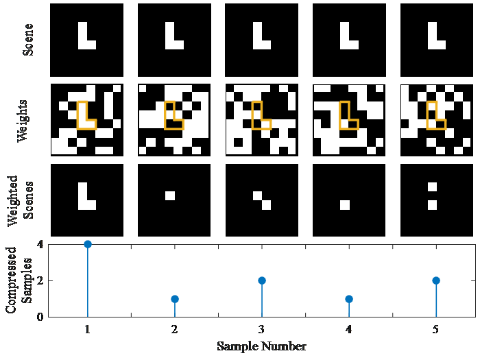
Figure 5: Each Column Illustrates One Compressed Measurement (Source: CCDC ARL).
The bottom plot shows the compressed sample produced by each column. For each measurement, the light of the weighted scene is focused on the single sensor, which sums all of the light and measures its intensity, producing a compressed sample. If the value of each black and white pixel of the weighted scene is 0 and 1, respectively, then the value of the compressed samples will be the number of white pixels in the weighted scene. The figure shows five example DMD patterns that produce five compressed samples. The samples themselves do not resemble the scene. But once enough samples have been taken, they can be processed by an optimization algorithm to recover an image of the scene.
Figure 6 shows the image from Figure 3 that used 512 x 512 = 262,144 pixels on the left compared to a simulated CS recovered image using 262,144 compressed samples on the right. This used the same method of taking compressed samples, as shown in Figure 5, except a 1024 x 1024 DMD was set to 262,144 different random patterns, producing 262,144 compressed samples. An algorithm processed these samples to produce a 1024 x 1024 image, with the “ARL” clearly visible. We have achieved a resolution of 1024 x 1024 using 4x less measurements, beating the Nyquist-Shannon sampling rate! This example illustrates the essential components of CS. Compressed samples are formed as randomly-weighted sums of the signal, typically requiring some form of specialized hardware. These samples are then postprocessed to reconstruct the original signal using fewer samples than predicted by traditional sampling theory.
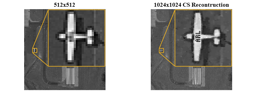
Figure 6: A Comparison of Traditional Sampling (Left) and CS (Right) (Source: CCDC ARL).
Sparsity
The Nyquist-Shannon sampling theorem states that the sampling rate must be at least twice the highest frequency of the signal—equivalently, the pixel width cannot be larger than the smallest feature of the scene. The sampling rate depends on the highest frequency of the signal. In CS, the number of measurements required depends on the sparsity of the signal, not its highest frequency. The sparsity of a signal is inversely proportional to its number of nonzero elements. Sparse signals are mostly close to 0, with a relatively few number of larger nonzero values. Remarkably, CS works well as long as the signal is sparse in any basis, not just the standard basis. For example, the 1 + 10 Hz signal in Figure 1 shown in the time domain is not sparse, i.e., most of the values are not 0. However, when the signal is represented in the Fourier basis (frequency domain), as in the top left of Figure 2, there are only two nonzero values, making it very sparse. Many naturally-occurring signals are sparse in some basis, allowing CS to be applied to a variety of applications. CS worked in the airport image because images are generally sparse in bases such as the 2-D Fourier or 2-D wavelet.
The left plot of Figure 7 shows a normal image in the standard basis. The middle plot shows this image in the wavelet basis, with the amplitude shown in a log scale for emphasis. The right plot compares the sparsity of the image in the standard and wavelet. For this 256 x 256 image, all 65,536 pixel values were arranged in descending order to create the line labeled “Original.” The same was done for the image in the wavelet basis and labeled “Wavelet.” Just like the 1 + 10 Hz signal, even though the image is not sparse in the standard basis, it is sparse in the wavelet basis. The important point is that the sparser the signal, the better CS works, i.e., the signal can be reconstructed with less measurements. Higher-dimensional signals, such as three-dimensional (3-D) images, are typically very sparse, making them ideal candidates for CS.
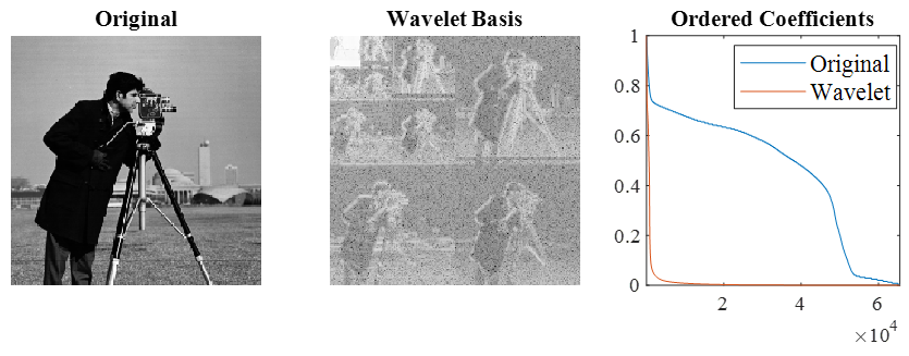
Figure 7: Comparison of an Image in Standard and Wavelet Bases (Source: CCDC ARL).
Incoherence
In the single-pixel camera example, the DMD was used to produce randomly-weighted sums of the data. The weights do not have to be random; they just have to be incoherent with the sparse basis of the data. Incoherence can be thought of as maximally different. For example, when using a Fourier basis, the pattern of weights should be as different as possible from the sinusoids of the Fourier basis. It happens to be that completely random weights are incoherent to any basis, but pseudorandom or structured weights can also be used in CS. Using CS theory, these weights can be optimized to achieve maximum performance [21], but they also have to be realizable in hardware. For example, a DMD cannot produce arbitrary valued weights. The mirrors can only point two directions, away or toward the sensor, resulting in weights of 0 or 1. Depending on the hardware used to implement the CS weights, the weight values may have limitations that affect CS performance.
Data Reconstruction
A detailed description of CS reconstruction algorithms is outside the scope of this article, but there are a few relevant points to mention. In traditional sampling, a signal can be perfectly reconstructed if it is sampled above the Nyquist rate. Similarly, in CS, a signal can be perfectly reconstructed if there are enough measurements relative to its sparsity. Real signals are not perfectly sparse, i.e., many of the values will be close to 0 but not actually 0. If these values are small enough, however, they will have minimal impact on CS performance.
The distinction between signal noise and measurement noise is important in CS. Measurement noise is created in the measurement process, e.g., electronic noise in the sensor. Signal noise is present in the signal being measured before it reaches the sensor, e.g., external interference. Signal noise is frequently measured as a signal-to-noise ratio (SNR), where a low SNR indicates a noisy signal. CS performs well in the presence of measurement noise. Reconstruction remains stable, with the quality of the reconstruction proportional to the noise level. CS performs poorly, however, when the signal has a low SNR [22]. Unfortunately, the CS process itself can degrade the SNR. In order to reconstruct the original signal, the random weights used to make the compressed measurements must be known. For example, the states of the DMD in the single-pixel camera must be known for each measurement and used in the reconstruction algorithm. In an ideal case, this information is known perfectly and is not a source of error. In practice, movement or miscalibration will introduce error, decreasing the signal’s SNR and hampering CS.
The number of measurements needed to produce an accurate reconstruction is proportional to the sparsity of the data. However, the exact sparsity of the data is not known a priori. Therefore, practical systems have to be designed for worst-case scenarios, increasing the required number of measurements. Another important consideration is that the optimization algorithms that reconstruct the data are very computationally intensive. Progress has been made to accelerate these algorithms [23], but they can still hamper real-time applications or systems with limited computing resources.
Compressive Sensing vs. Compression
CS is related to compression. When data is compressed, a large quantity of data is represented by a smaller amount of data. Typically, the full, uncompressed data is acquired first before a compression algorithm reduces it to a manageable size. For example, in traditional imaging, high-resolution imagers capture every pixel of an image and then throw away most of the data as it is compressed into a JPEG format. On the other hand, CS uses specialized hardware to compress the data at the time of measurement. Only the compressed measurements are saved; nothing is thrown away. From this viewpoint, CS is more efficient than typical imaging practices. CS can be used directly on data as a compression algorithm, independent of any sensor system. But traditional compression algorithms generally perform better than CS when the full data set is already available.
Compressive Sensing vs. Inpainting
In some cases, CS can be confused with inpainting [24]. Typically, inpainting refers to filling in the missing samples of an image, but it can also refer to filling in the missing samples of other types of data. Inpainting works with traditional samples, it does not use weighted sums of the data. Missing samples can occur accidently due to occlusions, noise, or damage; or nonuniform sampling can be done on purpose. Inpainting is confused with CS because CS reconstruction algorithms can also be used for inpainting. The main result of CS—that sparse data can be perfectly reconstructed using a small number of compressed samples—does not apply to inpainting. This is why CS is a much more powerful tool than nonuniform sampling for enhancing sensor systems.
Case Studies
Single-Pixel Camera
The single-pixel camera can be viewed as an application of CS to increase measurement speed or, alternatively, image resolution. A scanning camera that measures 1 pixel at a time would require 1024 x 1024 measurements to create a 1024 x 1024 image. A CS architecture using 4x less measurements would decrease the acquisition time by a factor of 4. Alternatively, a scanning camera using a 512 x 512 DMD would take the same amount of time to acquire an image as a 1024 x 1024 CS camera. However, the CS camera would have a resolution 4x higher than the scanning camera. Although CS can significantly increase the measurement speed or resolution of a scanning camera, there are several reasons why the single-pixel camera might not be a commercial success. They are as follows:
- Even if CS can increase measurement speed, it may not increase it enough to be practical for many applications.
- Given the long measurement time, camera or subject motion may introduce noise that impacts the reconstruction results.
- The effectiveness of CS is related to the sparsity of the data. Even though 2-D images are generally sparse, they may not be sparse enough to make this application practical.
- The cost of traditional short-wave IR (SWIR) cameras has been decreasing [25]. In addition, the DMD mirrors are limited to the near IR and SWIR range, preventing application to mid- wave IR, long-wave IR (LWIR), and far IR (FIR) imaging. These factors limit the marketability of a DMD-based solution.
InView has been developing technology to address some of these problems, such as using multiple sensors to decrease measurement time [26] and hyperspectral cameras that target sparser 3-D data sets [27]. But at this time, it appears that InView has not made large inroads into the IR imaging market.
Cell Phone Camera
Another CS imaging application is in low-powered, complementary metal-oxide semiconductor (CMOS) imagers [28]. Instead of using CS for measurement speed or resolution, this application focuses on reducing power. Each pixel in a typical 2-D imaging array is made up of a light sensor that produces a voltage and an ADC that converts the analog voltage to a digital value. This is illustrated in Figure 8 on the left with an example 4 x 4 imager. For a 1024 x 1024 sensor, each image requires about 1 million analog to digital (A/D) conversions. Multiplying that by the number of images needed for a video results in significant power usage, especially for mobile devices with limited battery life.
CS can be used to reduce power consumption by reducing the number of A/D conversions required for each image. Compressed samples are produced by connecting each ADC to a random pattern of sensors, requiring less A/D conversions per image (as illustrated in Figure 8 on the right). The problem with this approach is the image reconstruction. CS image reconstruction takes time and computing resources, probably using more power than initially saved. This CS imager would only be useful in a niche application where the video is not needed in real time and can be reconstructed in postprocessing using powerful computers. It would certainly be undesirable as a cell phone camera.
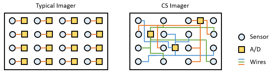
Figure 8: Comparison of a Typical CMOS Imager and CS Low-Power CMOS Imager (Source: CCDC ARL).
Magnetic Resonance Imaging
The only truly successful commercial application of CS is possibly the MRI [29, 30]. MRI detects radio frequency emissions from tissue excited by magnetic fields. Due to the physics of the system, measurement takes place in the Fourier basis, requiring a basis change back to the standard basis to retrieve the image. Figure 9 shows a simple example of a 2-D MRI, which is similar to the 1 + 10 Hz, 1-D signals in Figures 1 and 2. The first plot on the left in Figure 9 shows an image in the standard basis composed of low- and high-frequency 2-D sinusoids. A real MRI might depict an image of a brain. The next plot shows the image in the Fourier basis. The white dot in the lower left represents the low-frequency 2-D sinusoid shown in the third plot, while the grey dot in the upper left represents the high-frequency sinusoid in the last plot. A typical MRI system would scan through the Fourier basis, acquiring all of the points at the desired sampling rate. Once all of the Fourier samples are taken, they can be transformed to the standard basis to retrieve the image.
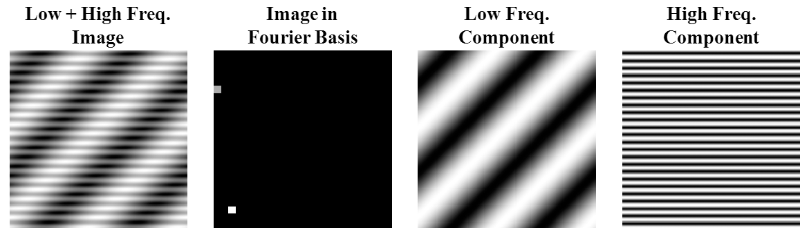
Figure 9: A Simple MRI Example (Source: CCDC ARL).
The amplitude of the points in the Fourier basis corresponds to the correlation between the sinusoid represented by that point and the image. This is calculated by the sum of the image multiplied by that sinusoid. For example, the amplitude of the white point is the sum of the image multiplied by the sinusoid in the third plot. Thus, each traditional MRI sample in the Fourier basis is really a compressed sample—a weighted sum of the image, where the sinusoids act as the weights. This means that CS can be applied to MRI without any hardware changes. Using CS theory, a fraction of the full number of samples typically required for MRI can be used to reconstruct an image, significantly reducing measurement time. MRI CS has a number of advantages [31]. They are as follows:
- MRI is often used to produce 3-D data (e.g., Figure 10). Higher-dimensional data is typically sparser than lower-dimensional data, enabling 3-D MRI to benefit more from CS than 2-D imaging applications.
- MRI imaging is performed in a high-SNR laboratory environment.
- No new hardware is required to produce the compressed samples. Flexible hardware that can be programed with arbitrary weights would be ideal, but MRI that uses Fourier weights has worked well in practice [32].
- There is substantial motivation for increasing the speed of MRI. Patients are required to remain still for long periods of time, which can be difficult in many instances. In addition, MRI equipment is very expensive. Increasing the throughput of an MRI machine will decrease overall cost.
- Image reconstruction can easily be done using powerful computers in postprocessing. Real-time image reconstruction is not required.
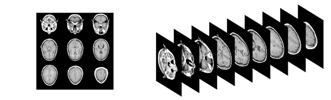
Figure 10: Example 3-D MRI as a Grid (Left) and Stacked (Right) (Source: CCDC ARL).
Guidelines
The following five positive aspects of applying CS to MRI can be formulated as general conditions for the successful application of CS.
- The data should be very sparse; higher-dimensional data is ideal.
- The SNR should be high; a laboratory environment is ideal.
- The hardware that produces the incoherent weights needed for CS should be easily available.
- There must be substantial motivation for adopting a CS strategy so the benefits outweigh any disadvantages.
- The application must be able to accommodate the long reconstruction time and high computing costs of CS.
It is possible to use CS in a case that does not satisfy these conditions, but it will be more difficult to produce a practical system. We will try applying these guidelines to two test cases to determine their suitability for a CS implementation. The first application is an IR imager for spinning munitions (shown in Figure 11) [33]. The scene is projected through the coded aperture onto the sensors to create weighted samples. The coded aperture is a randomly-patterned mask that blocks random sections of light from reaching the sensor. The coded aperture pattern cannot be changed like the mirrors of a DMD, but the rotation of the aperture relative to the scene via the natural rotation of the munition can produce the different weights for each compressed sample. The coded aperture shown in Figure 11 has a relatively low resolution for illustration purposes. In practical applications, the resolution of the coded aperture is much higher than the sensor array, increasing the resolution of the sensor array the same way the DMD increases the resolution of a single sensor. We apply the guidelines as follows:
- Two-dimensional data is only moderately sparse.
- A high-dynamic munition flying through the sky will not have a high SNR.
- The rotating, coded aperture produces semistructured weights not ideal for CS.
- High-resolution IR imagers are expensive, motivating the use of CS to increase the resolution of inexpensive low-resolution imagers.
- A munition imager for target recognition must operate in real time, although there may be ways to use compressed CS data without reconstruction [34].
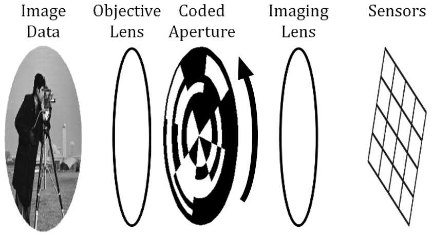
Figure 11: Architecture of a CS IR Imager for Spinning Munitions (Source: CCDC ARL).
Only the fourth guideline is encouraging. The cost benefits of CS must be weighed against the cost of the CS hardware and other disadvantages associated with it. Clearly applying CS in this case would be challenging.
Another possible CS application is antenna pattern measurement [35]. Figure 12 shows an example antenna pattern as a blue line around an antenna under test (AUT). A traditional measurement system is shown on the left. The circle of dots around the AUT represent test antennas that transmit one at a time (green), while the others are inactive (red). The sensitivity of the AUT is measured relative to each test antenna, creating an antenna pattern. The middle plot shows a CS implementation where random patterns of test antennas transmit simultaneously.
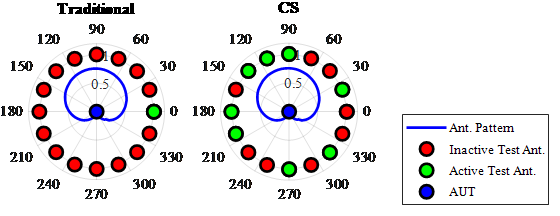
Figure 12: Comparison of Traditional and CS Antenna Pattern Measurement (Source: CCDC ARL).
The transmissions are summed in the AUT, creating a compressed sample. The CS implementation reduces the number of measurements required, accelerating the measurement process. We can show that the following five conditions apply, making this a promising application of CS:
- Antenna patterns are often 3-D (azimuth, elevation, and radio frequency) and therefore very sparse.
- Measurement is typically performed in a controlled laboratory environment with high SNR.
- There are already systems that use multiple test antennas placed in a ring around the AUT to measure antenna patterns. These systems could be easily modified to activate random combinations of these antennas instead of using them one at a time. The on/off patterns of test antennas are similar to the on/off patterns created by a DMD, which work well for CS.
- Antenna pattern measurement is typically an expensive, slow procedure, giving substantial motivation to use CS to accelerate measurement by reducing the number of samples.
- There is no problem postprocessing the data; the data are not needed in real time.
Conclusions
Now that we know what CS is and have examined some case studies, we can answer the questions raised in the Introduction.
- Many unsubstantiated comments about CS are simply untrue. CS is not “linear interpolation, rebranded.” The example of signal reconstruction using traditional sampling in Figure 2 is a form of interpolation. CS uses an optimization algorithm to identify signal coefficients in a sparse basis from compressed samples. This is not interpolation.
- The claim that CS is not new is somewhat true. Sources trace the history of CS as far back as 1795 to Prony’s method [7]. More recent results include Fadil Santosa and William Symes in 1986 [36], but it was not until 2006 that David Donoho coined the term “compressive sensing” [37]. Since then, Donoho and others have advanced CS theory and championed its use in the measurement process. No matter how new CS theory really is, the widespread push to use it to improve a variety of sensor systems is new.
- The claim that CS is overhyped is probably true. Even CS researchers acknowledge that “…compressed sensing has not had the technological impact that its strongest proponents anticipated” [9]. When reading about all of the applications of CS, it may seem that CS is revolutionizing many sensor technologies. However, most of these applications are experimental systems that have not overtaken traditional techniques. For example, when Wikipedia states that “compressed sensing is used in a mobile phone camera sensor” [2], it is not talking about all phone cameras. It is referring to the experimental low- power CMOS imager in the case study that was never actually used in any commercial cell phone.
- Open criticism of CS from researchers such as Leonid Yaroslavsky and Kieran Larkin [11, 12] partially stem from the overhyped publicity of CS. Their comments can be generally understood to say that CS will not provide the best performance in all cases, and, in many practical situations, more traditional sampling or compression strategies will outperform CS. This is certainly true. On the other hand, CS has achieved significant results that will increase performance for certain applications. CS does deserve recognition, as well as further research and funding, even if it is not the panacea some have claimed.
- An additional point is that the growth in CS has also advanced topics, such as the properties of random matrices, sparse representation, and optimization algorithms applicable to areas outside sensing and measurement. Even if CS sensor hardware has been slow to develop, there are many related fields benefiting from CS research.
Can CS solve your sensor and measurement problems? As with most significant questions, there is not an easy yes or no answer. CS is definitely not a cure-all that can be used in every situation. The fact that Mark Neifeld declared that “we haven’t discovered the ‘killer’ application yet” [10] when accessing the potential of CS imagers with leaders in the defense sector should give one pause if they think that their application is the “killer” application. The five guidelines listed are a good starting point. CS should realistically be compared to other alternatives, whether with other sampling techniques such as basis scanning [38] or alternate sensor technologies. CS results that seem promising in idealized settings might not perform well in more realistic scenarios. CS is still developing. An application that is not practical in the near term might still deserve longer-term research. Government and industry leaders should approach CS with their eyes open. They should be aware of the advantages and disadvantages of CS and know if the funded research is practical and short term or more theoretical and long term. In 1956, there was a surge in optimism about information theory much like the hype CS is experiencing. The words of Claude Shannon, of the Nyquist- Shannon sampling theorem, ring true today as much as they did then [39].
Information theory has, in the last few years, become something of a scientific bandwagon… What can be done to inject a note of moderation in this situation? In the first place, workers in other fields should realize that the basic results of the subject are aimed in a very specific direction… A thorough understanding of the mathematical foundation and its …application is surely a prerequisite to other applications. The subject of information theory has certainly been sold, if not oversold. We should now turn our attention to the business of research and development at the highest scientific plane we can maintain… A few first-rate research papers are preferable to a large number that are poorly conceived or half finished.
Whether CS can solve your problem or not, there is a final lesson to learn from CS methodology. The hardware and software aspects of sensor systems should not be designed independently, rather there should be an interdisciplinary codesign resulting in an optimal solution [8].
References
- Elad, M. “Sparse and Redundant Representation Modeling—What Next?” IEEE Signal Processing Letters, vol. 19, no. 12, pp. 922–928, 2012.
- Compressed Sensing, https://en.wikipedia.org/wiki/Compressed_sensing.
- Duarte, M. F., et al. “Single-Pixel Imaging Via Compressive Sampling.” IEEE Signal Processing Magazine, vol. 25, no. 2, pp. 83–91, 2008.
- Why Compressive Sensing Will Change the World, https://www.technologyreview.com/s/412593/why-compressive-sensing-will-change-the-world/.
- Uncompressing the Concept of Compressed Sensing, https://statmodeling.stat.columbia.edu/2013/10/27/uncompressing-the-concept-of-compressed-sensing/.
- Shtetl-Optimized: The Blog of Scott Aaronson, https://www.scottaaronson.com/blog/?p=3256.
- The Invention of Compressive Sensing and Recent Results: From Spectrum-Blind Sampling and Image Compression on the Fly to New Solutions with Realistic Performance Guarantees, http://vhosts.eecs.umich.edu/ssp2012//bresler.pdf.
- Strohmer, T. “Measure What Should Be Measured: Progress and Challenges in Compressive Sensing.” IEEE Signal Processing Letters, vol. 19, no. 12, pp. 887–893, 2012.
- Foucart, S., and H. Rauhut. “A Mathematical Introduction to Compressive Sensing.” Bull. Am. Math, vol. 54, pp. 151–165, 2017.
- Neifeld, M. “Harnessing the Potential of Compressive Sensing,” https://www.osa-opn.org/home/articles/volume_25/november _2014/departments/harnessing_the_potential_of_compressive_sensing/.
- Yaroslavsky, L. P. “Can Compressed Sensing Beat the Nyquist Sampling Rate?” Optical Engineering, vol. 54, no. 7, p. 079701, 2015.
- Larkin, K. “A Fair Comparison of Single Pixel Compressive Sensing (CS) and Conventional Pixel Array Cameras,” http://www.nontrivialzeros.net/Hype_&_Spin/Misleading%20 Results%20in%20Single%20Pixel%20Camera-v1.02.pdf.
- Candès, E. J., and M. B. Wakin. “An Introduction to Compressive Sampling [A Sensing/ Sampling Paradigm That Goes Against the Common Knowledge in Data Acquisition].” IEEE Signal Processing Magazine, vol. 25, no. 2, pp. 21–30, 2008.
- Baraniuk, R., et al. “An Introduction to Compressive Sensing.” Connexions E-Textbook, pp. 24–76.
- Willett, R. M., R. F. Marcia, and J. M. Nichols. “Compressed Sensing for Practical Optical Imaging Systems: A Tutorial.” Optical Engineering, vol. 50, no. 7, p. 072601, 2011.
- Rani, M., S. B. Dhok, and R. B. Deshmukh. “A Systematic Review of Compressive Sensing: Concepts, Implementations and Applications.” IEEE Access, vol. 6, pp. 4875–4894, 2018.
- Strohmer, T. “Measure What Should Be Measured: Progress and Challenges in Compressive Sensing.” IEEE Signal Processing Letters, vol. 19, no. 12, pp. 887–893, 2012.
- Gregg, M. “Compressive Sensing for DoD Sensor Systems.” JASON Program Office, MITRE Corp., Mclean, VA, No. JSR-12-104, 2012.
- Camera Chip Makes Already Compressed Images, https://spectrum.ieee.org/semiconductors/optoelectronics/camera-chip-makes-alreadycompressed-images.
- Toward Practical Compressed Sensing, http://news.mit.edu/2013/toward-practical-compressed-sensing-0201.
- Elad, M. “Optimized Projections for Compressed Sensing.” IEEE Transactions on Signal Processing, vol. 55, no. 12, pp. 5695–5702, 2007.
- Davenport, M. A., et al. “The Pros and Cons of Compressive Sensing for Wideband Signal Acquisition: Noise Folding Versus Dynamic Range.” IEEE Transactions on Signal Processing, vol. 60, no. 9, pp. 4628–4642, 2012.
- Kulkarni, A., and T. Mohsenin. “Accelerating Compressive Sensing Reconstruction OMP Algorithm With CPU, GPU, FPGA and Domain Specific Many-Core.” 2015 IEEE International Symposium on Circuits and Systems (ISCAS), IEEE, 2015.
- Compressed Sensing or Inpainting? Part I, https://nuit-blanche.blogspot.com/2010/05/compressed-sensing-or-inpainting-part-i.html.
- Tech Trends: Thermal Imagers Feeling the Shrink, https://www.securityinfowatch.com/video-surveillance/cameras/night-vision-thermal-infrared-cameras/article/11152180/everything-about-infrared-technology-is-decreasing-including-size-and-most-importantly-cost.
- Kelly, K. F., et al. “Decreasing Image Acquisition Time for Compressive Imaging Devices.” U.S. Patent 8,860,835, 14 October 2014.
- Russell, T. A., et al. “Compressive Hyperspectral Sensor for LWIR Gas Detection.” Compressive Sensing, vol. 8365, International Society for Optics and Photonics, 2012.
- Oike, Y., and A. El Gamal. “CMOS Image Sensor With Per-Column ΣΔ ADC and Programmable Compressed Sensing.” IEEE Journal of Solid-State Circuits, vol. 48, no. 1, pp. 318–328, 2012.
- Lustig, M., D. L. Donoho, and J. M. Pauly. “Sparse MRI: The Application of Compressed Sensing for Rapid MRI Imaging.” Magn. Reson. Imaging, vol. 58, no. 6, pp. 1182–1195, 2007.
- Siemens Healthineers: Compressed Sensing, https://www.siemens-healthineers.com/en-us/magnetic-resonance-imaging/ clinical-specialities/compressed-sensing.
- Foucart, S., and H. Rauhut. “A Mathematical Introduction to Compressive Sensing.” Bull. Am. Math, vol. 54, pp. 151–165, 2017.
- Krahmer, F., and R. Ward. “Beyond Incoherence: Stable and Robust Sampling Strategies for Compressive Imaging.” Preprint, 2012.
- Don, M. L., C. Fu, and G. R. Arce. “Compressive Imaging via a Rotating Coded Aperture.” Applied Optics, vol. 56.3, pp. B142–B153, 2017.
- Davenport, M. A., et al. “The Smashed Filter for Compressive Classification and Target Recognition.” Computational Imaging V., vol. 6498, International Society for Optics and Photonics, 2007.
- Don, M. L., and G. R. Arce. “Antenna Radiation Pattern Compressive Sensing.” The 2018-2018 IEEE Military Communications Conference (MILCOM), IEEE, 2018.
- Santosa, F., and W. W. Symes. “Linear Inversion of Band-Limited Reflection Seismograms.” SIAM J. Sci. Statist. Comput., vol. 7, pp. 1307–1330, 1986.
- Donoho, D. L. “Compressed Sensing.” IEEE Trans. Inform. Theory., vol. 52, no. 4, pp. 1289–1306, 2006.
- DeVerse, R. A., R. R. Coifman, A. C. Coppi, W. G. Fateley, F. Geshwind, R. M. Hammaker, S. Valenti, and F. J. Warner. “Application of Spatial Light Modulators for New Modalities in Spectrometry and Imaging.” Spectral Imaging: Instrumentat., Applicat. Anal. II, vol. 4959, pp. 12–22, 2003.
- Shannon, C. E. “The Bandwagon.” IRE Transactions on Information Theory 2.1, vol. 3, 1956.
Biography
MICHAEL DON is an electrical engineer for ARL, where he specializes in high-performance embedded computing, signal processing, and wireless communication. He began his career as an intern at Digital Equipment Corporation, performing integrated circuit design for their next-generation Alpha processor, the fastest processor in the world at that time. After graduating, he worked for Bell Labs, where he engaged in the mixed-signal design of read channels for their mass storage group. Mr. Don holds a bachelor’s degree in electrical engineering from Cornell University and is currently pursuing a Ph.D. in electrical engineering at the University of Delaware, where he is researching compressive sensing applications for guided munitions.