


Introduction
Long-range radar systems designed to provide precise range measurements may, in certain cases, experience degraded tracking performance in range, which tends to negate the benefit of the designed sensor precision. The measurement uncertainty associated with long-range radar systems results in two major practical difficulties. First, when a system is tracking multiple targets closely spaced in a given region, the problem of assigning target measurements to existing tracks becomes more difficult, which may cause the radar to assign the wrong measurements to the wrong target and/or cause targets to be missed. Second, the estimation performance of the track filter employed by the radar processor may be degraded to the extent that the range reported by the filter is less accurate than the range reported by the raw measurements. In this case, the benefit of using a track filter is to a large extent negated.
The degraded tracking performance of long-range radar systems is due to the non-Gaussian nature of their measurement distribution when converted to Cartesian space. This distribution is often referred to as a “contact lens” or “banana” distribution due to its resemblance to these shapes in Cartesian space.
Current Methdos of Addressing Non-Gaussian Measurement Distributions
In almost all real-world radar systems, measurements are performed in polar (two-dimensional) or spherical (three-dimensional) coordinates of range and angles (or angle sines). The transformations from these coordinate systems to the Cartesian coordinates in which target dynamics are described are nonlinear. Most radar-tracking algorithms make use of some form of the well-known Kalman filter algorithm, which guarantees optimal performance given linear state dynamics and measurement models.
Popular modifications, such as the Extended Kalman Filter (EKF) and Unscented Kalman Filter (UKF), may also be used to address real-world state dynamics and measurements with mild nonlinearities, resulting in reasonable (but suboptimal) performance. All of these methods rely on approximating the state and measurement uncertainties as Gaussian distributions with a known mean and covariance parameter, as the process of Bayesian updates for Gaussian distributions can be conveniently performed using closed-form equations rather than numerical integration.
In many cases, the nonlinear target dynamics can be effectively addressed by employing the linearization techniques of the EKF or UKF. However, under certain conditions, the measurement transformations become sufficiently nonlinear to the extent that a Gaussian distribution inadequately models the uncertainty region in Cartesian space.
In Lerro and Bar-Shalom [1], a metric known as “bias significance” was developed to quantify the curvature of a polar radar measurement for the two-dimensional problem. If the range and angle measurements are modeled by independent Gaussian uncertainties with means and variances ![]() and
and ![]() , respectively, and the transformation from polar to Cartesian space is given by
, respectively, and the transformation from polar to Cartesian space is given by![]() and
and ![]() , then the bias significance (CB) is given by
, then the bias significance (CB) is given by
![]() .
.
Empirical results from Lerro and Bar-Shalom [1] suggest that if ![]()
 , then a standard linearization may be used without significant error. For values exceeding this number, adjustments are required to remove bias in the distribution mean and inflate the covariance.
In addition to the difficulties with mean and covariance, when the bias significance is high, the distribution takes on a highly non-Gaussian shape, resembling a banana (or, in three dimensions, a contact lens), and more sophisticated techniques must be employed to represent the distribution accurately.
Figure 1 illustrates this situation. The left and right diagrams depict a two-dimensional transformed measurement distribution for values of CB = 0.1 and CB = 1, respectively, along with the distribution means and covariances. The covariances are plotted as ellipses over the 3-sigma region in each eigen-axis. (For a Gaussian distribution, this represents the region containing approximately 99% of the distribution mass.) For the measurement depicted on the left, the region inside the covariance ellipse indeed contains most of the distribution, as it is approximately Gaussian. For the measurement indicated on the right, with CB = 1, the covariance ellipse does not accurately represent the distribution limits, as the measurement distribution is highly non-Gaussian in Cartesian space. Portions of the distribution fall outside the ellipse, and large empty areas exist within the ellipse, presenting an opportunity for misassociation of measurements with other tracks or false alarms. Additionally, the inflated covariance in the range (horizontal) dimension results in degraded performance in range estimation.

Several potential solutions to this problem have been proposed by various authors. The Measurement Adaptive Covariance EKF (MACEKF) [2] is one method that evaluates the angle accuracy of the track and inflates the range variance of the measurements adaptively to preserve covariance consistency. This approach works well when the track has settled but sacrifices range performance early in the track due to covariance inflation.
The Consistency-based Gaussian Mixture Filter (CbGMF) [3] attempts to solve the problem by splitting the track into a Gaussian Mixture, where the individual Gaussian components of the mixture have a limited angular support in covariance, therefore reducing the effect of the nonlinearity. However, many track components are frequently needed to represent the track and guarantee consistency.
The Gaussian Mixture Measurement-Integrated Track Splitting (GMM-ITS) [4] filter instead splits the measurement into a Gaussian mixture to better represent the non-Gaussian nature of the distribution. However, the splitting method used does not preserve the covariance of the measurement distribution in range.
The work presented herein describes a new way to model radar measurements using a Gaussian mixture [5, 6]. Rather than using an ad hoc procedure for Gaussian mixture splitting, as performed in Tian et al. [3] and Zhang and Song [4], a Gaussian mixture that optimally models the measurement in an information-theoretic sense is generated. Furthermore, a method for intelligently choosing the number of mixture components that should be used to model a given measurement is provided. The proposed methodology will improve the performance of long-range radar tracking by allowing the full precision of the measurements to be captured.
Gaussian Mixture Distribution Models
A Gaussian mixture is defined as a weighted sum of Gaussian probability density functions (PDF). Let ![]() denote a Gaussian PDF. Then a general Gaussian mixture is given by
denote a Gaussian PDF. Then a general Gaussian mixture is given by
![]() ,
,
where ωk are the component weights, μk are the component means, and Σk are the component covariances. For a single-Gaussian model, the mean and covariance may be chosen to specify the distribution. On the other hand, a Gaussian mixture model provides a much larger number of parameters to be chosen.
One strategy of matching a Gaussian mixture to an arbitrary PDF is to attempt to match higher-order moments, as was done by Pearson [7], but the closed-form solutions associated with this approach quickly become unmanageable. In Tian et al. [3] and Zhang and Song [4], the strategy is to reduce the degrees of freedom by artificially restricting the covariances of the components to be equal, positioning the component means at equal intervals around the distribution mean, and then choosing the weights based on the likelihood of the means under the original distribution.
Our approach to choosing the distribution parameters is to attempt to optimize the distance between the mixture and the true distribution in an information-theoretic sense. The “distance” to be minimized is known as the Kullback-Leibler (KL) divergence, defined as
![]() ,
,
where p(x) is the true distribution and q(x) is the model distribution. This integral is essentially the expected value of the log likelihood ratio of the true distribution to the model distribution, with expectation taken over the true distribution.
In a practical sense, KL divergence describes the ease with which two distributions may be distinguished by log likelihood testing. If the KL divergence is low, then differences between them may only be discerned by examining the log likelihood evaluated over a large number of samples.
For discrimination applications, it is usually desired to maximize KL divergence between discrimination class distributions to more easily distinguish them from each other by log likelihood testing. However, in our application, the distributions should be as similar as possible so that when the measurement likelihood is used to update the PDF of the state, it provides a good representation of the true likelihood function. Therefore, to provide a “good” match of the Gaussian mixture model distribution q(x) to the true measurement p(x), the number of Gaussians NG and the parameters ωk,μk,Σk should be chosen such that KL divergence is limited.
A single-Gaussian model of a polar radar measurement converted to Cartesian coordinates matched in mean and covariance to the true distribution has KL divergence ![]() . This is the minimum KL divergence that may be achieved by a single-Gaussian model. This equation provides a direct relationship between bias significance and KL divergence.
. This is the minimum KL divergence that may be achieved by a single-Gaussian model. This equation provides a direct relationship between bias significance and KL divergence.
Numerical Optimization of Distribution Parameters
The KL divergence integral for the Gaussian mixture optimization involves the log of a sum that is difficult to analyze in closed form. Therefore, numerical optimization methods must be employed to choose the parameters. Given a set of samples of the true measurement distribution p(x), the Expectation Maximization (EM) algorithm [8] can be applied to estimate a set of parameters, which minimizes KL divergence between the mixture and the distribution samples.
If a sufficiently large sample size is used and/or Monte-Carlo runs of the process are performed, an excellent estimate may be obtained of the optimal parameters needed to model the measurement distribution with a mixture of a given size. Additionally, the KL divergence achieved by the mixture approximation is provided by the final output of the EM algorithm.
This process generates a mixture model for a measurement with a given mean range and angle and their associated measurement variances. However, without some transformation of the results, this computationally intensive fitting process would have to be run for each distinct set of measurement input parameters, or equivalently a large (four-dimensional) lookup table of values stored for each mixture size desired.
A recent Georgia Tech Research Institute (GTRI) discovery makes this method practical: For an EM mixture parameter fit of given size NG with a fixed bias significance CB , regardless of individual parameters, the final KL divergence obtained is approximately invariant. (This approximation holds effectively for σθ << 1 rad.) Additionally, the component weights ωk produced by the solution process are also the same. This suggests that the means μk and covariances Σk may also be transformed in such a way that the results are the same if the bias significance is held constant. The KL divergence achieved by these fits is shown in Figure 2.
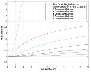
Based on Lerro and Bar-Shalom [1], it is known that a single-Gaussian model with linearized mean and covariance estimates performs poorly above CB = 0.2. This situation is corroborated by the KL divergence curve shown for the First-Order Single-Gaussian Model. An improvement in performance may be realized up to about CB = 0.5 by using a properly moment-matched single-Gaussian model, but beyond this value, the Gaussian mixture models provide a much better level of performance.
This research determined that the following transformations of the component means and covariances resulting from EM are constant if the bias significance and number of Gaussian components are held constant. Let [μk ]x and [μk ]y represent the x and y Cartesian components of the component means. First, transform the Cartesian mean to polar coordinates.
![]() .
.
Then normalize these polar coordinates as follows:
![]() .
.
For the covariance, perform an eigendecomposition of Σk such that ![]() is the major axis eigenvalue (corresponding to cross-range variance for the long ranges involved in the contact lens problem) and
is the major axis eigenvalue (corresponding to cross-range variance for the long ranges involved in the contact lens problem) and ![]() is the minor axis eigenvalue (corresponding to range variance). Furthermore, let ψk be the angle of the major eigen-axis measured counterclockwise from the x-axis. Then transform this eigendecomposition as follows:
is the minor axis eigenvalue (corresponding to range variance). Furthermore, let ψk be the angle of the major eigen-axis measured counterclockwise from the x-axis. Then transform this eigendecomposition as follows:
![]() .
.
The quantities ![]() , along with the KL divergence achieved by the solution, may now be placed into a lookup table, where the rows of the table are measurement bias significance, CB, and number of components, NG. This lookup table has only one unique dimension for a given number of mixture components (rather than four), resulting in a much more tractable implementation.
, along with the KL divergence achieved by the solution, may now be placed into a lookup table, where the rows of the table are measurement bias significance, CB, and number of components, NG. This lookup table has only one unique dimension for a given number of mixture components (rather than four), resulting in a much more tractable implementation.
For an arbitrary measurement (subject to σθ<<1 rad), a Gaussian mixture may then be generated by the following steps:
Compute the bias significance, ![]() .
.
Consult the lookup tables to determine the KL divergence that may be achieved by using a given number of mixture components to model the measurement.
Choose the lowest number of components, NG, required to achieve the desired KL divergence.
Look up ![]() from the table for the given NG and CB.
from the table for the given NG and CB.
Perform the inverse of the transformations described previously to compute ![]() .
.
Model Results
To demonstrate the effectiveness of this measurement modeling approach, Monte-Carlo simulations of the lookup-table-based mixture generation process were performed over a logarithmic grid of angle standard deviations from 1 to 300 mrad and bias significances from 0.3 to 10 (which in turn determine the range standard deviation). A fixed range of 100 km was used. The KL divergence from the lookup table (predicted) was compared to the empirical KL divergence calculated by sampling the original polar measurement distribution with 1 million points, converting these points to Cartesian coordinates, and calculating the expectation of the log likelihood.
Figure 3 shows the result of this analysis for NG=3 components. The predicted KL divergence agrees well with the lookup-table measurement model over the domain of interest. Some slight deviation on the order of 0.01 is observed in the lower bias significance portions of the grid. This deviation is partly due to sampling error, as well as the fact that KL divergence is plotted on a log scale.

Figure 4 illustrates one of these three-component mixture densities in comparison to the true distribution. This figure shows that the mixture distribution represents the shape of the measurement PDF much more closely than a single-Gaussian ellipse. These results may be compared to Figure 5, which shows results for NG=5 components. Again, some slight discrepancies on the order of 0.01 are present at low bias significance values. The KL divergence achieved here is lower (as can be seen by comparison to Figure 2), so sampling error effects can be seen at a higher CB than in Figure 3. However, the lookup-table-based mixture models still achieve close to the expected KL divergence performance over the entire domain of interest.


Conclusion
As the popularity of high-range-resolution, long-range radars continues to increase, the tracking difficulties associated with these systems continues to be a problem for operators, designers, analysts, and other practitioners dependent on these types of radar results. However, the novel method described herein addresses this problem by modeling two-dimension polar radar measurements in Cartesian coordinates using a Gaussian mixture distribution. This method has already demonstrated some promising preliminary results when applied to tracking filters [5, 6], and developers are in the process of conducting research to extend this approach to three-dimensional monostatic and bistatic radar measurements as well.
References:
- Lerro, D., and Y. Bar-Shalom. “Tracking With Debiased Consistent Converted Measurements Versus EKF.” IEEE Transactions on Aerospace and Electronic Systems, vol. 29, pp. 1015–1022, 1993.
- Tian, X., and Y. Bar-Shalom. “Coordinate Conversion and Tracking for Very Long Range Radars.” IEEE Transactions on Aerospace and Electronic Systems, vol. 45, pp. 1073–1088, 2009.
- Tian, X., Y.Bar-Shalom, G. Chen, K. Pham, and E Blasch. “Track Splitting Technique for the Contact Lens Problem.” 2011 Proceedings of the 14th International Conference on Information Fusion (FUSION), pp. 1–8, 2011.
- Zhang, Q., and T. L. Song. “Gaussian Mixture Measurements for Very Long Range Tracking.” 12th International Conference on Informatics in Control, Automation and Robotics (ICINCO), pp. 457–464, 2015.
- Davis, B., and W. D. Blair. “Gaussian Mixture Approach to Long Range Radar Tracking With High Range Resolution.” 2015 IEEE Aerospace Conference, pp. 1–9, 2015.
- Davis, B., and W. D. Blair. “Adaptive Gaussian Mixture Modeling for Tracking of Long Range Targets.” 2016 IEEE Aerospace Conference, Big Sky, MT, 2016.
- Pearson, K. “Contributions to the Mathematical Theory of Evolution.” Philosophical Transactions of the Royal Society of London. A, vol. 185, pp. 71–110, 1894.
- Bilmes, J. A. “A Gentle Tutorial of the EM Algorithm and Its Application to Parameter Estimation for Gaussian Mixture and Hidden Markov Models.” International Computer Science Institute, vol. 4, p. 126, 1998.