


A DATA EXPLOSION
From the edges of the observable universe to medical image scanners on Earth, there is an ever-growing need to quickly process and understand large amounts of audio and visual data. Audio data capture a wide range of frequencies, for example; and human speech patterns are incredibly complex and extremely diverse. Similarly, visual data come in many forms, including video sequences, images from multiple cameras, medical scanners, etc. And recent trends with big data have produced large quantities of labeled data from which interesting patterns have yet to be discerned and used. Not surprisingly, processing such data in situ at interactive rates without significant hardware requirements is one major challenge arising from the big data revolution.
Applications in a variety of domains require accurate and robust processing of these types of data to achieve specific goals. One of the most common problems is image recognition, in which a solver must identify main objects of interest in image data. The demand for faster and more accurate image recognition algorithms has led to the development of several image recognition databases and contests, of which the ImageNet Large Scale Visual Recognition Challenge (ILSVRC) is the most well-known [1].
Figure 1 shows accuracy trends for ILSVRC contest winners over the past several years. Whereas traditional image recognition approaches employ hand-crafted computer vision classifiers trained on a number of instances of each object class, in 2012 Alex Krizhevsky entered a deep neural network (DNN), now known as AlexNet, that reduced the error rate of the next closest solution by more than 10% [2]. By 2015, the winning ILSVRC algorithm rivaled human capabilities, and today deep learning algorithms exceed human capabilities.
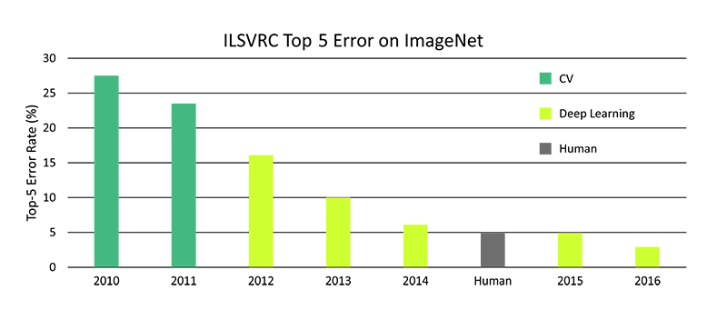
Figure 1: ImageNet Top-5 Classification Error Over Time.
The success of AlexNet is regarded by many as the genesis of deep learning’s resurgence [3]. While notionally deep learning has existed in various forms since the early 1980s, only recently have deep learning algorithms become computationally practical. Modern graphics processing unit (GPU) architectures, now explicitly designed for deep learning algorithms, have enabled many of the recent and impressive achievements of contemporary deep learning techniques.
At the same time, these massively parallel architectures are driving the next generation of deep learning algorithms for intelligent video analytics (IVA). IVA broadly categorizes events, attributes, or patterns of behavior in video data. For example, automatic target recognition (ATR) defines the process of identifying and localizing an object in an image (e.g., a person in the top-left corner of the image). ATR capabilities also extend to event detection (such as isolating a person running) and path analysis (such as determining how people cross a busy intersection). These capabilities combine to create systems capable of providing intelligent, actionable insights to human users.
One system that is being built to leverage many of these advancements is Sentinel™. Developed by the SURVICE Engineering Company in Belcamp, MD, this system (which is discussed in detail later) combines state-of-the-art techniques in high-performance computing (HPC), modern data reduction and analysis techniques, and deep learning to realize ATR, tracking, event detection, and other visually oriented tasks. These components combine to create a flexible, scalable system for improved situational awareness in a variety of intelligence, surveillance, and reconnaissance (ISR) scenarios.
DEEP LEARNING
The possible applications of modern deep learning are both wide and deep. Recently, deep learning has been applied successfully to problems in representation learning. For example, a variety of factors influence every single piece of data in many real-world classification problems: a picture of a red car in broad daylight will contain red pixels, whereas a picture of that same car at night will exhibit nearly black pixels. Deep learning solves the representation learning problem by building complex representations (wheels or headlights) from simpler concepts (edges, color, and so forth) [4].
One common example of a deep learning model is the feedforward DNN. Originally inspired by biological neuron models, this DNN is composed of artificial neurons, which take some number of inputs and produce a single output. Perhaps the first artificial neuron was the perceptron [5], which produced a simple binary output from simple binary inputs. Modern neurons are often modeled on sigmoid functions, which produce an output in the range [0,1] given inputs in the same range. Neurons combine to form a network comprising (possibly) several layers, where each layer has some number of neurons and each neuron is fully connected to the subsequent layer.
Figure 2 illustrates a typical DNN. On the left side of the figure is an example artificial neuron, which takes some number of inputs to produce a single output. There exist many types of artificial neurons, but the most common are compute sigmoid, linear rectified, or hyperbolic tangent functions. On the right side is an example artificial neural network (NN). NNs are typically composed of several layers. The leftmost layer in this network is called the input layer, and the neurons within the layer are called input neurons. The rightmost, or output, layer contains the output neurons. The middle layers are called hidden layers, as neurons in this layer are neither strictly inputs nor strictly outputs. A neural network may contain many hidden layers; DNNs are those networks comprising more than one hidden layer.
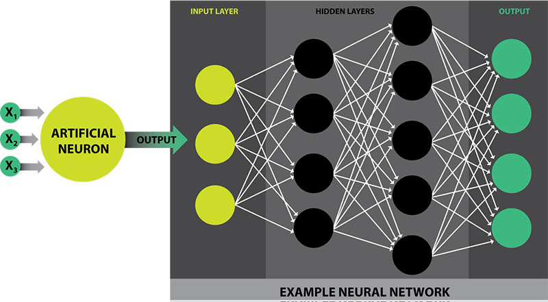
Figure 2: DNNs for Learning Applications.
DNN applications generally employ a two-phase approach. In the offline, or learning, phase, the network ingests large quantities of labeled data to learn some desired task. This type of learning is known as supervised learning. For example, a network attempting to recognize images of cats or dogs would ingest a collection of images with labels indicating whether each picture contains a cat or a dog. The network topology is organized such that the number of output layers corresponds to the number of object classes—in this case, two. Each network node is initialized with a random weight, which is then refined by repeatedly exposing the network to images of cats or dogs. Weights are adjusted through a process known as backpropagation [4] until the correct node is activated—that is, until the output node value corresponds to either “cat” or “dog.”
The online, or inference, phase consists of simply passing data elements through the previously trained network. Continuing the previous example, the trained network might ingest a picture of a cat not encountered during training. Given a sufficiently diverse training set, the network generalizes the features underlying the new image to infer that the picture does, in fact, depict a cat.
Convolutional Neural Networks (CNNs)
With increased DNN performance on massively parallel computing architectures (generally) and modern GPUs (specifically), advances in the field have seen performance in ATR tasks rivaling human capabilities [6]. This increase in accuracy is achieved by augmenting traditional DNNs operating on image data with convolution layers that learn to recognize more complex visual features. These improved networks (an example of which is shown in Figure 3) are called CNNs.
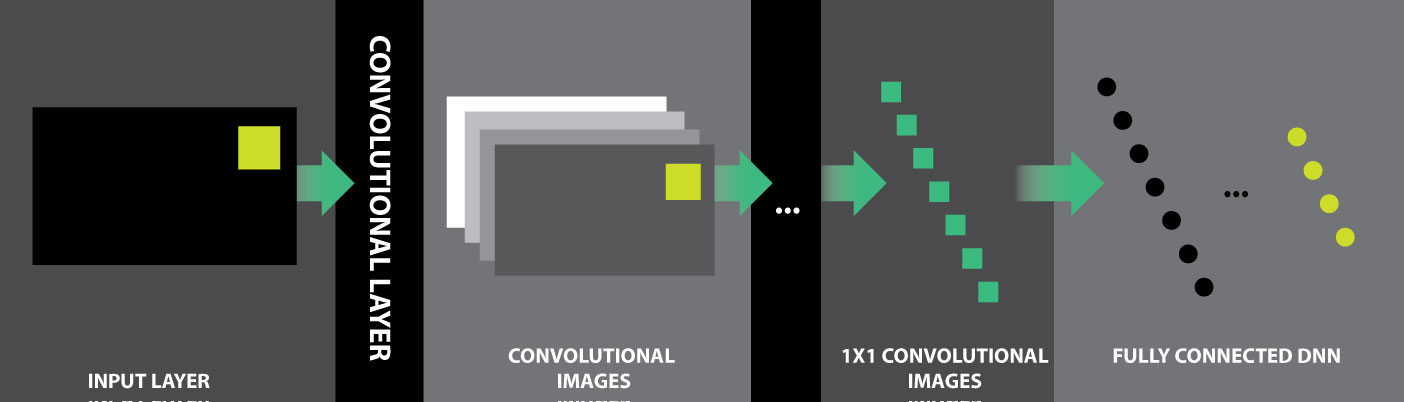
Figure 3: CNN Example.
To recognize more complex visual features in images, convolutional layers in CNNs apply convolution kernels to each pixel in the input (image) layer. A convolution kernel is a matrix of values encoding weights that are applied to the operating pixel’s nearest neighbors. For example, convolution kernels are used extensively in image processing to sharpen or to blur images. In this case, kernel weights are learned by the network. A convolutional layer thus produces a set of images to which the kernel has been applied. The number and size of the convolutional images vary based on the kernel size and overall network topology. Often, this process is applied repeatedly until convolutional images comprising a single pixel are obtained. These 1×1 images then serve as input to a fully connected DNN, which ultimately performs the desired task.
While CNNs are applicable to a wide variety of scenarios, the availability of large, labeled data sets for image recognition has increased the efficacy of CNNs for recognition tasks. For example, these networks power image-based searches and often serve as the visual systems for robotic systems. Recently, NVIDIA demonstrated BB8, a CNN-based autonomous car. The CNN was trained using only 72 hr of human driving data—captured by two forward-facing cameras—and performs exceptionally well in similar, but not exactly identical, driving environments [7]. The ability to generalize underlying features to correctly perform a desired task, as in autonomous driving with NVIDIA’s BB8, demonstrates the potential power of CNNs for artificial intelligence (AI) applications.
Recurrent Neural Networks (RNNs)
Success with CNNs in visually oriented applications have spurred advances in audio applications as well. In typical CNN topologies, current inference tasks do not enhance the network’s recognition abilities in future tasks. While this lack of impact is not a major concern for certain visual tasks—for example, identifying a cat in an image—information derived from new examples can be highly useful for speech recognition tasks. So-called recurrent networks, or those in which current inference tasks inform future tasks, are the key mechanism behind recent success in speech-to-text recognition applications based on deep learning.
Recurrent neural networks (RNNs) are named for their cyclic topology—namely, the addition of recurrent, or latent, network layers connecting to previous layers. This topology permits current inference tasks to influence the network’s performance in future tasks. A schematic of a typical recurrent network topology is illustrated in Figure 4. Note that the particular size, position, and number of recurrent layers vary depending on desired outcomes, but the simple network above demonstrates the fundamental topology. Here the yellow layer cycles back to a previous layer, providing new information based on the data it processes.
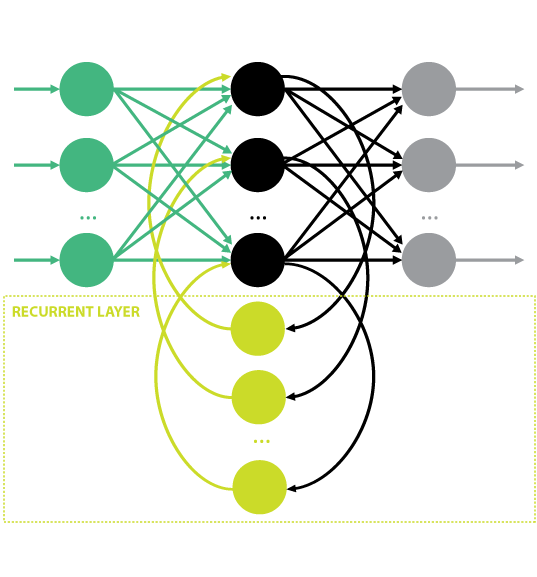
Figure 4: RNN Example.
A major challenge in speech recognition is the wide variability in human speech patterns, as well as the presence of background noise. Recently, Baidu Research demonstrated excellent performance with a type of RNN known as long short term memory (LSTM) networks. The second iteration of Baidu Research’s system, Deep Speech 2, implements NNs trained with the Connectionist Temporal Classification loss function to predict speech transcriptions from audio [8]. Deep Speech 2 has been trained on 11,940 hr of English and 9,400 hr of Mandarin, and the system works quite well for multiple languages [8]. The ability to use new information derived from current processing tasks—advanced speech recognition, in this case—provides insight into the potential power of RNNs.
DNN Organization and Computational Requirements
After witnessing significant advances in the application of CNNs to a wide variety of machine learning problems, several organizations have created software frameworks supporting deep learning research and development. For example, Microsoft provides the Computational Network Toolkit (CNTK) [9], and Google offers TensorFlow [10].
CNTK, TensorFlow, and similar deep learning frameworks provide mechanisms for building NNs, allowing creation of traditional feedforward DNNs, CNNs, and even LSTM networks. To support a variety of topologies, these frameworks structure NNs as directed graphs in which each leaf node represents an input value or parameter and each interior node represents a matrix operation over its children. Such graphs are called computational networks. The computational network in Figure 5 represents a one-hidden-layer sigmoid NN. Generally speaking, the concept of layers as introduced previously is not used in the computational network structure, but the simpler network description tends to enable greater flexibility.
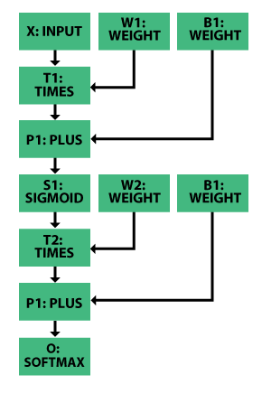
Figure 5: Example Network Encoding One-Hidden-
Layer Sigmoid Network.
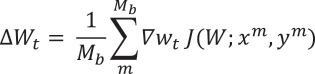
Training requires a cost function to evaluate network accuracy. Numerous possibilities exist, but popular criteria include cross-entropy for classification [9] and mean-square error for regression tasks [9]. In CNTK, for example, the computation network model parameter, W, is improved at each step, t, as:
![]() ,
,
where
 ,
,
and Mb is the mini-batch size, which increases optimization performance. The gradient computation for ![]() is accelerated by storing partial derivatives at model parameter nodes. The network is optimized using a stochastic gradient descent [9] during backpropagation to effectively update W for correct output in an incremental manner. Agarwal et al. [9] provide a complete description of the gradient calculation for various nodes in CNTK.
is accelerated by storing partial derivatives at model parameter nodes. The network is optimized using a stochastic gradient descent [9] during backpropagation to effectively update W for correct output in an incremental manner. Agarwal et al. [9] provide a complete description of the gradient calculation for various nodes in CNTK.
In the online phase, when model parameters (that is, weight nodes in Figure 5) are known, inference simply requires sequential execution of each vertex in the graph: each node provides an input and an operation to produce its output. When multiple nodes are coupled together, this simple execution model implements advanced NN capabilities.
However, training NNs is difficult on traditional HPC architectures—for example, central processing unit (CPU) clusters—because of significant communication between compute nodes. When the entire network is instead trained on a single GPU, communication latency is reduced, bandwidth is increased, and both physical size and power consumption of compute resources are significantly decreased, particularly when compared to CPU clusters. For example, stochastic gradient descent, a simple but effective training algorithm, executes as much as 40 times faster on a GPU compared to a CPU [3].
This substantial difference results directly from the structure of computational networks: these networks are massively parallel structures, comprising thousands or millions of identical units, each performing the same computation on different data. Importantly, most of these units exhibit no interdependence and can thus be computed simultaneously—that is, in parallel. This execution model, the data-parallel single instruction, multiple data (SIMD) model, matches precisely the underlying hardware architectures of modern GPUs.
GPUs FOR DEEP LEARNING
Recently, NVIDIA has made significant strides in GPU computing for deep learning applications, in both desktop and mobile hardware spaces. For example, the NVIDIA DGX-1 Deep Learning System is powered by Tesla 100 accelerators and trains AlexNet using 1.28 million images with 90 epochs (iterations) in approximately 2 hr [2]. In contrast, a CPU-only implementation requires more than 6 days to train AlexNet under the same conditions.
NVIDIA’s Telsa 100 accelerators are based on their newest architecture, Pascal, and are designed specifically for deep learning and AI applications. The Pascal architecture boasts native 16-bit floating point support, resulting in significant speedups for deep learning algorithms. Memory is fast, Chip-on-Wafer-on-Substrate (CoWoS) with High Bandwidth Memory 2 [11], which enables vertical stacking of multiple memory dies. The net result of these architectural features is faster memory accesses than previously achievable. At the same time, connectivity in multi-GPU systems is increased by NVLink, which enables GPU-to-GPU transfers at rates up to 160 GB/s of bidirectional bandwidth. The Telsa P100 GPU boasts 3584 CUDA cores (more than 15 billion transistors) operating at a base clock speed of 1,328 MHz. These extreme capabilities provided by the Pascal architecture enable high-performance DNN training.
In the mobile space, NVIDIA’s Tegra line of processors enables fast online inference with trained networks on low-cost and low-size, -weight, and -power (SWaP) CUDA-enabled hardware. For example, NVIDIA’s Jetson TX1, which NVIDIA hails to be “the world’s first supercomputer on a module,” is designed for compute-intensive embedded applications and features an NVIDIA Maxwell GPU with 256 CUDA cores, 4 ARM A57 CPUs with SIMD processing support via ARM NEON extensions, 4K video encode and decode capabilities, and a camera interface capable of 1,400-MP/s throughput. This system is designed for the latest NVIDIA deep learning inference engine, TensorRT, which is used to rapidly optimize, validate, and deploy trained NNs for AI-powered applications. As shown in Figure 6, Jetson TX1 is roughly the size of a credit card, which allows easy coupling to mobile platforms supporting a wide variety of deployment scenarios, from small unmanned aerial vehicles to large armored vehicles.
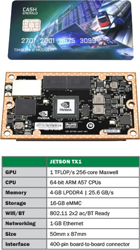
Figure 6: NVIDIA’s Tegra X1 Mobile GPU Platform.
SENTINEL
As mentioned previously, Sentinel is a system that is being developed by the SURVICE Engineering Company to leverage all of these advancements and provide real-time in situ IVA. The system exploits proven methods for data reduction and analysis; object localization, detection, and recognition; and advances in modern computing architectures to support human-in-the-loop deployment scenarios with application to ISR problems in defense, homeland security, disaster relief, emergency response, and even home security. Despite tremendous progress in both hardware and software support, next-generation computer vision and data analysis systems—such as Sentinel—place high demands on the resources supporting their implementation. The challenges inherent to these systems must be overcome to realize real-time in situ IVA for augmenting and enhancing users’ understanding of live data streams.
To exploit the benefits of modern GPUs, programmers must understand and use data-level parallelism carefully and correctly, which is often a difficult and time-consuming task. However, with careful consideration of the low-level architectural features, the SIMD units of modern GPUs offer potentially significant increases in runtime performance across the full range of GPU computing platforms.
For example, as shown in Figure 7, initial results with dynamic mode decomposition (DMD) for foreground/background separation within Sentinel demonstrate significantly better-than-real-time performance [12]. At the same time, Sentinel’s ATR capabilities exploit current computational network frameworks to instantiate proven CNN topologies for state-of-the-art detection. Specifically, the system uses the Inception-v3 topology [13] for ATR, capitalizing on the latest GPU computing frameworks to accelerate both training and inference. Integrating these frameworks in Sentinel permits high-performance CNN training on desktop- and workstation-class systems, with trained networks deployed across the full range of NVIDIA GPUs, including its Tegra mobile computing line.
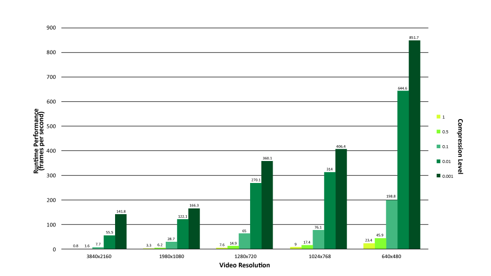
Figure 7: Sentinel DMD-Based Foreground/Background Separation.
Sentinel Performance, NVIDIA Tesla K40c
The performance and flexibility of Sentinel also permits a distributed architecture to support various deployment scenarios. In particular, in situ IVA processing uses the NVIDIA Tegra X1 hardware platform coupled with commercial-off-the-shelf (COTS) sensor hardware to execute core data analysis operations onboard, so that only relevant, actionable information need be transmitted to the primary user interface. As summarized in Figure 8, this distributed architecture enables Sentinel-enabled IVA modules to execute remotely. For example, a Sentinel-enabled IVA module mounted on a UAV can relay customizable battlefield information not only to forward-deployed units but also to analysts or operators at a central location, ultimately resulting in informed decisions regarding possible courses of action.
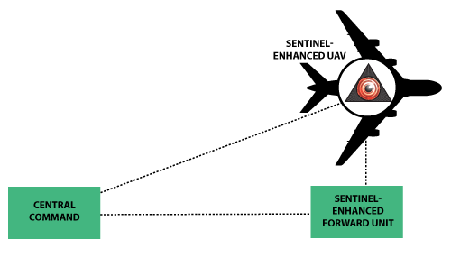
Figure 8: Distributed Architecture Enabling Diverse Operations for Sentinel-Enabled Modules.
Real-time in situ IVA provided by the core Sentinel computer vision and data analysis system enables informed decisions based on enhanced understanding of live data streams. At the same time, the distributed architecture allows Sentinel-enabled IVA applications to span a continuum, from fully centralized for traditional analysis tasks on desktop system, to fully distributed for aerial ISR and other remote sensing scenarios.
Pushing computation to mobile computing architectures has many advantages, particularly in cases where multiple live video streams or other sensor data are monitored in parallel. A distributed architecture reduces computational requirements at centralized locations and reduces total system failure rates by decoupling system components. In addition, sending only relevant information derived from Sentinel-processed data streams across networks reduces overall communications traffic. These capabilities offer the potential to reduce users’ cognitive burden and, ultimately, to improve decision-making in many military and commercial ISR scenarios.
FUTURE IMPACT
The increased efficacy of deep NNs in both image and speech recognition tasks, coupled with increased performance via GPU acceleration, has brought about a resurgence of deep learning techniques. NVIDIA’s recent hardware and supporting software frameworks enable the next generation of deep learning applications, such as demonstrated in the Sentinel real-time, in situ intelligent video analytics system. The distributed architecture enables diverse deployment scenarios, ultimately providing means to transmit only relevant, actionable information to interested parties.
Continued advancements and refinements in deep learning may serve as the foundation to high-level task planning AI systems. Already, CNNs control automobiles in a wide variety of driving scenarios—from markerless roads to construction zones to busy highways—while speech recognition systems power companion AI applications on cell phones and other low-cost, low-SWaP platforms. Current deep learning achievements are both important and significant; however, these techniques nevertheless require additional research, development, and, ultimately, coupling with human-like cognitive AI architectures to enable the next-generation applications supporting the modern warfighter.
References:
- Russakovsky, O., J. Deng, H. Su, J. Krause, S. Satheesh, S. Ma, Z. Huang, A. Karpathy, A. Khosla, M. Bernstein, A. C. Berg, and L. Fei-Fei. “ImageNet Large Scale Visual Recognition Challenge.” IJCV, 2015.
- Krizhevsky, A., I. Sutskever, and G. E. Hinton. “Imagenet Classification with Deep Convolutional Neural Networks.” Advances in Neural Information Processing Systems, 2012.
- Nemire, B. “CUDA Spotlight: GPU-Accelerated Deep Neural Networks.” https://devblogs.nvidia.com/parallelforall/cuda-spotlight-gpu-accelerate…, accessed May 2016.
- Goodfellow, I., B. Y. and A. Courville. Deep Learning. MIT Press, 2016.
- Rosenblatt, F. “The Perceptron – A Perceiving and Recognizing Automaton.” Cornell Aeronautical Laboratory Report, 1957.
- He, K., X. Zhang, S. Ren, and J. Sun. “Delving Deep into Rectifiers: Surpassing Human-Level Performance on ImageNet Classification.” Microsoft Research, 2015.
- Bojarski, M., D. Del Testa, D. Dworakowski, B. Firner, B. Flepp, P. Goyal, L. D. Jackel, M. Monfort, U. Muller, J. Zhang, X. Zhang, J. Zhao, and K. Zieba. “End to End Learning for Self-Driving Cars.” 2016.
- Baidu Research. “Deep Speech 2: End-to-End Speech Recognition in English and Mandarin.” Silicon Valley AI Lab, 2015.
- Agarwal, A., E. Akchurin, C. Basoglu, and G. Chen. “An Introduction to Computational Networks and the Computational Network Toolkit.” Microsoft Technical Report MMSR-TR-2014-112, 2014.
- Abadi, M., A. Agrawal, P. Barham, and E. Brevdo. “TensorFlow: Large-Scale Machine Learning on Heterogeneous Systems.” Google Whitepaper, 2015.
- NVIDIA. “NVIDIA Tesla P100.” NVIDIA White Paper, 2016.
- Tu, J. H., C. W. Rowley, D. M. Luchtenburg, S. L. Brunton, and K. J. Nathan. “On Dynamic Mode Decomposition: Theory and Applications.” Journal of Computational Dynamics, vol. 2, pp. 391–421, 2014.
- Szegedy, C., V. Vanhoucke, S. Loffe, J. Shlens, and Z. Wojna. “Rethinking the Inception Architecture for Computer Vision,” arXiv1512.00567, 2015.